WiFi-based Local Positioning System

This is a project writeup of some experiments in building a WiFi-based localization system around my apartment. AirTags use similar principals but are not WiFi-based.

Mapping the Area

Positioning starts with mapping so you can know where you are in the space.

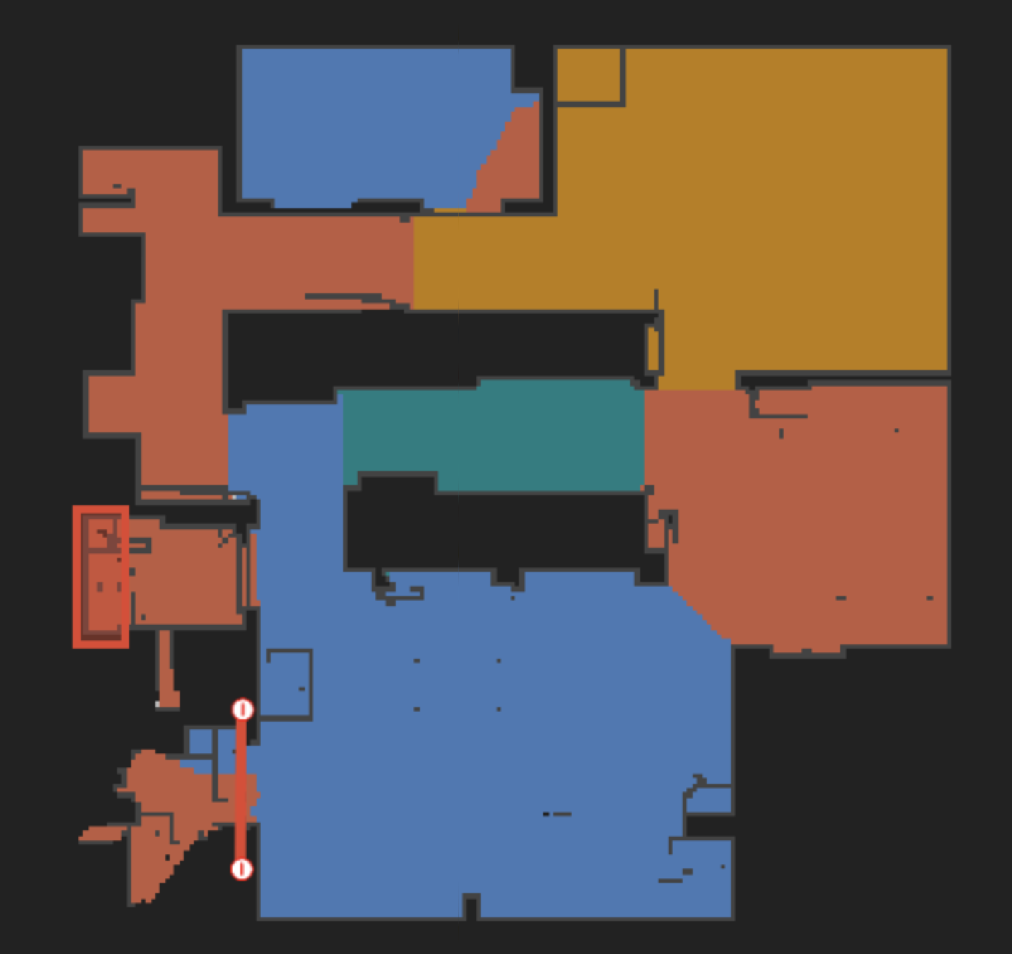
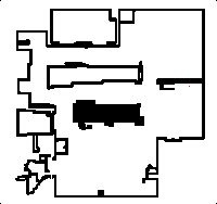
I have a Roborock robot vacuum that's mapped my apartment. Unfortunately, without using Valetudo, I can't download any rich map data. So the only map data source is the screen capture of the map in the app. Starting with that app map screenshot, a little processing in GIMP removed the no-go zones, room bounds, and small objects that created obstructions in the map. I kept some of the obstructions since they are useful "geographical features" for localizing in larger empty spaces. Applying low brightness and high contrast filters created the clean map.

→

The good thing about a map from a robot vacuum is that it provides a highly accurate representation of the actual floor plan. Other tools like mobile apps that do augmented-reality mapping where you point your camera and place a point at the corner of each wall have higher error and need manual correction afterwards. Pixels on this map are directly proportional to physical distances, making it really easy to do a transformation between the map space and the physical space.

Building a Baseline

With a map at hand, it's time to build a layer on top of the map with the signal strength of the surrounding WiFi networks. The signal layer is used to trilaterate the position of our device.

Assuming a gradient where the strongest signal strength is at the WiFi router location with equal signal loss in all directions: data from a single WiFi network would yield a circle of possible locations, two networks yields two points, and three networks yields a single point. WiFi does degrade with obstructions like walls, microwaves, and anything metal (e.g. faraday cages). But in a relatively static environment that signal degradation should not change over time.

The below images shows signal data for three network. The points indicate sample locations. The gradient shows the interpolated signal strength. The first two (red and green) are controlled WiFi signals. The third (blue) is not. The signal strength is measured is negative decibels, meaning a lower value is a higher signal strength.

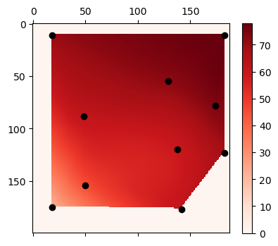
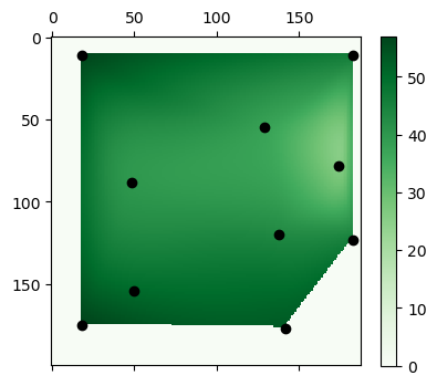
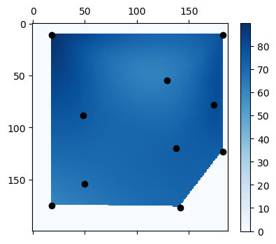
The signal maps above were generated with the code below. Interestingly, scipy's libraries for interpolation only interpolates in the interior space between points. It doesn't extrapolate data outside the outer hull.

import numpy as np
import scipy as sp
import pandas as pd
import matplotlib.pyplot as plt
import imageio

map_positions = {
    "green_origin": (174, 78),
    "red_origin": (18, 175), # also bottom_left
    "bottom_right_bottom": (142, 177),
    "bottom_right_right": (183, 123),
    "upper_left": (18, 11),
    "upper_right": (183, 11),
}

house_map_img = imageio.imread('map.png')
house_map = np.asarray(house_map_img)

data = pd.read_csv("data.csv")
# data is read from a CSV with 3 columns: {SSID, Location, Strength}

def show_for_ssid(filter_ssid):
    values_raw = sorted(
        [
            tuple(r) for r in
            data[data["SSID"]==filter_ssid]
                .filter(items=["Location", "Strength"])
                .to_numpy()
        ],
        key=lambda x: map_positions[x[0]]
    )
    points = list(map(lambda x: map_positions[x[0]], values_raw))
    values = list(map(lambda x: x[1], values_raw))

    interp = sp.interpolate.CloughTocher2DInterpolator(
        points,
        values,
        fill_value=0
    )

    X_orig = np.linspace(0, house_map.shape[0], house_map.shape[0])
    Y_orig = np.linspace(0, house_map.shape[1], house_map.shape[1])
    X, Y = np.meshgrid(X_orig, Y_orig)
    Z = interp(X, Y)

    plt.matshow(Z, cmap=cm)
    plt.plot(*list(zip(*points)), "ok")
    plt.colorbar(shrink=0.8)
    plt.show()

    return X, Y, Z

X, Y, Z1 = show_for_ssid("RED", plt.cm.Reds)
_, _, Z2 = show_for_ssid("GREEN", plt.cm.Greens)
_, _, Z3 = show_for_ssid("BLUE", plt.cm.Blues)

Preparing for Trilateration

With the data collected, the question becomes: can this data be to trilaterate location? Unfortunately, the answer is "Yes, but...".

The base way to calculate location is to treat signal strength as a proxy for distance. Then use the three "distances" to construct the "three circles" and find the single intersecting point (or with the least amount of error if there is no single shared point between all three).

This doesn't work here because signal strength is actually non-linear. It can't be used 'in-place' of distance, and would need to be converted to actual distance. That isn't so difficult since there is enough data to build a gradient.

The other (big) problem with this method is that not all the WiFi station locations are known. The data collected comes from two controlled stations (red, green) and one uncontrolled station (blue).

An alternative that doesn't require either a linear distance function (although it would benefit from it) or station locations known beforehand is to find the position that most closely matches the interpolated gradient of the signals.

Before implementing this, it's important to verify that there is enough "signal" in the signal to clearly distinguish pixels. There are a few ways to calculate this -- a statistical pixel comparison or calculating the gradient's derivative to find flat or unchanging spots. The former probably has the benefit of being a global measure of similarity and the latter, a local one.

I opted to do something much simpler -- manual verification. The three gradients are used as the individual RGB layers of an image. Any "flat" spots in the signal gradient with lots of similarity without change (which corresponds to the derivative) are likely very similar. The below image shows the RGB combination of the three signal layers above.

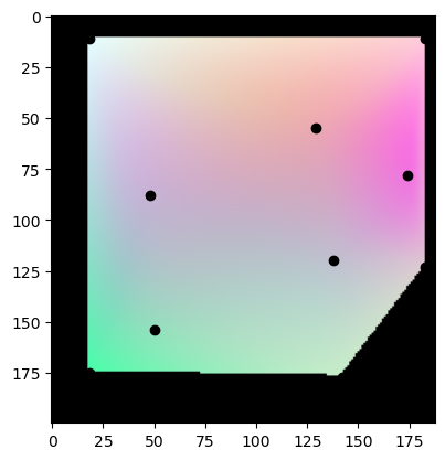
The gradient hotspots seems to be focused around the points, but that may not be a bad thing as points selected for data capture were chosen (not very scientifically) because they would be unique. This is acceptable for a basic test run. Although in a future iteration of this project, it might be interesting to do some outlier detection to verify the integrity of this test.

Trilateration

With the signal gradient covering the entire space and confirmation that we have enough uniqueness across the space to identify specific points, we can trilaterate by running a simple "classification" task that finds the point closest in signal against a sample signal.

def trilateralate(sample_data):
    def norm_data(Z):
        return (Z - 20) / (100 - 20)

    map_shape = Z3.shape
    Z = np.stack((Z1, Z2, Z3), axis=2)

    point_matrix = np.repeat([[point_data]], map_shape[0], axis=0)
    point_matrix = np.repeat(point_matrix, map_shape[1], axis=1)

    diff = np.absolute(norm_data(Z) - norm_data(point_matrix))
    diff_sum = np.sum(diff, axis=2)
    diff_min_point = np.where(diff_sum == np.min(diff_sum))

    return diff_min_point

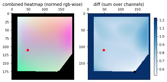
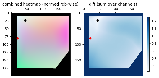
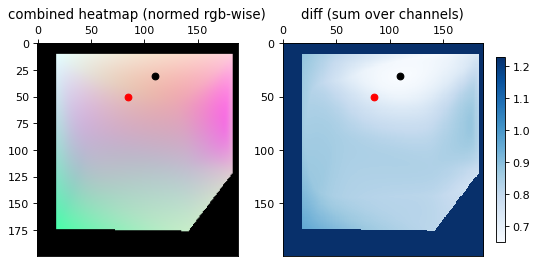
Results

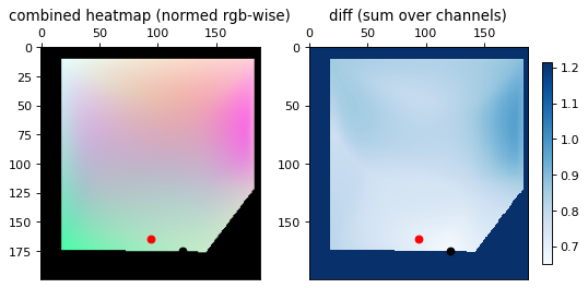
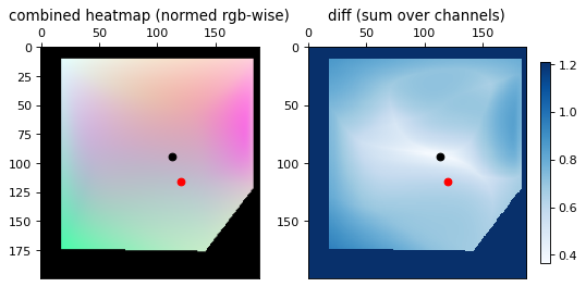
The images below show the results for several samples. The red dot represents the ground truth and the black dot represents the trilaterated result. The left image is the placement on the same RGB heatmap seen above. The right image is the diff between the RGB heatmap and the current point, from which the minimum point is found.

There is a high error, but the general region that the signal trilaterates to is correct. The appropriate room could be identified and even the right general area of the room, but there could be no meaningful precision with the high error rate.

Conclusion

Trilateration works. Although I consider this project done, a few areas to improve on:

1. More data to build a better gradient. And more efficient ways to passively collect the ground-truth signal data.
2. Multi-device experiments. I have no idea how well this carries over to other devices (beyond the two controlled signal sources and my phone).
3. More than 3 signals used in "regression" and "classification" pieces. I'd expect better precision, but the strength of other signals would be lower so that may not be the case.
4. Collecting many samples for a good statistics of signal error and trilateration error. It could also inform the quality of the gradient and improve the precision.
5. Easier data collection -- there's no app that provide direct-to-json formats for labeling. I'd need to DIY an Android application for this.